A.M.C. Davies
Norwich Near Infrared Consultancy, 10 Aspen Way, Cringleford, Norwich NR4 6UA, UK. E-mail: [email protected]
Introduction
I was introduced to Multiple Linear Regression (MLR) when I was a very junior laboratory assistant at Glaxo Laboratories in 1959. Glaxo were about to install their first computer (only the third commercial computer in the UK!) and they wanted to reassure the staff that it was not going to lead to redundancies. The emphasis was on what the computer could do that was currently impossible. They chose MLR as the demonstration and after 55 years, I can still visualise a scene from the cartoon-like film we were shown. A vast hall full of white-bearded mathematicians working with slide rules that the film explained would be required to compute an MLR computation, while the computer would take only a few hours! Since those days there have been many advances in computing and in regression analysis.
I first used MLR for real in 1966 when researching the factors involved in the crystallisation of honey. We had only a few variables and got some pleasing results. In 1980 I started work in near infrared (NIR) spectroscopy using an instrument with 19 filters and employing a programmable calculator to compute MLR calibrations. Perhaps I should refer to it more correctly as S for Step-wise MLR. My first problem was that the program could handle only 12 variables, so the initial task was to select 12 out of 19 variables. A problem we never really did solve except by using those filters which were known to have absorptions in the analyte being studied. We rapidly moved to using real computers, having first to modify the programs to utilise 19 variables, but there were still difficulties. Obtaining an apparently useful result was not a problem, but trying to find stable solutions was very difficult. About this time I first met my friend and collaborator, Tom Fearn, who was working with chemists using a similar NIR filter instrument. Tom wrote a program for discovering the “best-pair” of filters which worked pretty well. In1982 I persuaded my Institute to buy an NIR grating instrument which produced a spectrum from 1100 nm to 2500 nm measurements at 2 nm intervals; 700 variables! Now we did have problems! My first solution was to borrow Tom’s “best-pair program” but computing regression coefficients for 700 × 699 / 2 = 244,650 answers and trying to sort them was a big task for the small Nova 4 computer which ran the spectrometer. Instead we adopted a two-stage approach by computing a low resolution picture of variables at 40 nm intervals which produce 630 regression coefficients. These were displayed on a colour display (another first in the Institute) and an operator could then find areas of high correlation which were then computed at 2 nm intervals.1

When these were displayed, not only were we able to locate the variables which gave the best correlations but the shape of the surrounding correlations also indicated if they were likely to be stable. It took about 20 hours of processing time but it did work! However, we were rapidly over-taken by other developments.
The system was brought up-to-date by Tom Fearn as part of our course on matrix algebra.2 In its current MATLAB form it takes less than 5s to do the computations and display the results!
What are the problems with MLR?
I could produce a long list of problems associated with MLR, starting with: which of the many forms to use or how to assess the results. It is probably true that we should never have been using MLR or SMLR with NIR data because the data are highly correlated (sometimes known as collinearity) rather than being independent variables. However, it has to be said that Karl Norris (the “father of NIR analysis) has always used a special form of SMLR and was never beaten in the Chambersburg “Software Shootout”. His offer to become a judge of the contest was accepted so that there could be a new winner! It also has to be said that we have advanced to the present level of expertise because SMLR was available to get us started.
Advances in the MLR technique
Several techniques have been introduced which were all tackling the problem of collinearity. The most important are principal components regression (PCR) and partial least-squares (PLS) [it ought to be called PLS regression (PLSR) but this terminology is rarely used]. I attended the first international diffuse reflection conference (IDRC, normally called “Chambersburg”) in 1982 where I met Professor Fred McClure who introduced me to the use of Fourier transformation in NIR spectroscopy and we did some work in replacing NIR data with Fourier coefficients in process control3 but did not progress this work because I became fixed on another approach for utilising Fourier coefficients (CARNAC)4— more about this later in the year!
PCR was promoted by Ian Cowe5 and this will be discussed first because it is easier to understand PLS as a variation of PCR. In PCR the spectroscopic data is subjected to PCA and then the PCA scores are used in SMLR. The critical advantages of PCA are that the data are considerably compressed and they are orthogonal. Typically 700 NIR wavelength variables can be compressed into 20 PCs. The fact that PCA scores are orthogonal means that they are uncorrelated so the collinearity problem is removed. In Cowe’s work the PCs were selected, for regression, by their correlation with the analytical data but this has not been followed by all other workers. This meant that the PCs are selected by SMLR in the order of applicability and it is much easier to decide when to terminate the analysis.
PLS in the form that we use it was developed by Harald Martens and Svante Wold6 who took the original work by Herman Wold7 on problems in econometrics and social sciences and made it applicable to problems being tackled in chemometrics. PLS can most easily be understood by considering it as a modification of PCR. Like PCR, PLS computes new variables (always called factors in PLS) from the original data but with different criteria. PLS uses the variance of the data but it also takes into account the correlation of the data to the analytical values that we want to predict. In broad terms, in MLR the aim is to maximise R2, which can very easily give rise to over-fitting. In PCR the PCs are formed just by maximising the reduction in variance (V) while in PLS the new factors are selected by maximising the product of V and R2. Tom produced a MATLAB graphic that the operator could use to emulate these operations. The model worked with some random data x1, x2 and y. The random x data was plotted on the left-hand side of diagram and were projected on to a plane which provided values of z, for each point these data were plotted on the right-hand side of the diagram against the y values. As the plane is rotated by the operator the values of z change and this is continued until a maximum value is found for one of the three criteria, R2, V or V × R2. Pictures of these three maxima are shown in Figure 2.
 MLR optimises R2 but it produces an over-fitted result. (b) PCR produces a much more stable result by optimising V but with a reduced R2. (c) PLS also produces a stable result but with a slightly higher R2 by optimising V × R2.")
(a) A high value, 0.994, was achieved for R2 when just rotating to maximise it but (b) this fell to 0.698 when maximising V. A slightly higher value for R2 was obtained (c) when V × R2 was maximised. Why isn’t 0.994 the right answer? Of course it is for the diagram but if the data points were replaced with new values this value 0.99 would probably be considerably reduced and this is what happens with real data. The diagram only emulates the computation of the first PC for PCR and the first factor for PLS which provides the possibility that a calibration with good predictive performance and a high R2 can be discovered.
“What’s the point?”
Why am I labouring this topic? Do I think PLS should be abandoned? No, I would have preferred PCR to have been the chosen method because I think it is much easier to understand, but the development of PLS software is so superior this is not going to happen. Using PLS correctly, as we have demonstrated in several past issues, is much better than running MLR badly. However, I would like users to know that PLS is a development of MLR rather than a completely different “magical” algorithm. My suggestion is that people coming into this area should follow this course from MLR through PCR to PLS.
Acknowledgement
I am very grateful to Tom Fearn for the MATLAB GUI shown in Figure 2 and for all his work, advice and encouragement over the last 34 years.
References
- A.M.C. Davies, M.G. Gee and P.W. Foster, “A colour graphics display system to aid the selection of “best-pair” wavelengths for regression analysis of near infrared data”, Lab. Practice 33(5), 78–80 (1984).
- A.M.C. Davies and T. Fearn, “Doing it faster and smarter (Lesson 6 of matrix algebra)”, Spectrosc. Europe 14(6), 24 (2002).https://www.spectroscopyeurope.com/td-column/doing-it-faster-and-smarter-lesson-6-matrix-algebra
- A.M.C. Davies and W.F. McCLure, “Near infrared analysis in the Fourier domain with special reference to process control”, Anal.Proc. 22, 321 (1985). doi: http://dx.doi.org/10.1039/ap9852200321
- A.M.C. Davies and T. Fearn, “Quantitative analysis via near infrared databases: comparison analysis using restructured near infrared and constituent data-deux (CARNAC-D)”, J. Near Infrared Spectrosc. 14(6), 403–411 (2006). doi: http://dx.doi.org/10.1255/jnirs.712
- I.A. Cowe and J.W. McNicol, “The use of principal components in the analysis of near-infrared spectra”, Appl. Spectrosc. 39, 257 (1985). doi: http://dx.doi.org/10.1366/0003702854248944
- S. Wold, H. Martens and H. Wold, “The multivariate calibration problem in chemistry solved by the PLS method”, in Proc. Conf. Matrix Pencils March 1982, Lecture Notes in Mathematics, Ed by A Ruhe and B. Ka˙gström. Springer Verlag, Heidelberg, p. 286 (1983).
- H. Wold, “Soft modelling: The basic design and some extensions”, in Systems Under Indirect Observation, Causality-Structure Predictions, Ed by K.G. Jöreskog and H. Wold. North Holland, Amsterdam (1981).