Antony N. Daviesa,b Jan Gerretzena and Henk-Jan van Manena
aExpert Capability Group – Measurement and Analytical Science, Nouryon Chemicals BV, Deventer, the Netherlands
bSERC, Sustainable Environment Research Centre, Faculty of Computing, Engineering and Science, University of South Wales, UK
At a recent international conference, I attended a good lecture by a scientist using Ion Mobility Spectrometry (IMS) in a food analysis application. During the talk, one slide mentioned that they had used Savitzky–Golay smoothing on the IMS data and that started me wondering. I asked why they had decided that they needed to smooth the IMS data and was told that as they did it routinely for infrared spectra they just applied it to the IMS data as well.
I thought a better approach might have been to decide what data processing was really required and be able to justify the additional data manipulation steps in terms of improving on an analytical figure of merit, for example. You really need to start by accepting that the spectroscopic data you have just measured isn’t fit-for-purpose. Now measuring data of insufficient quality for the role it must play can have as many good (for “good” read unavoidable) reasons as bad.
Why is my raw data not fit-for-purpose?
One common reason is that you do not have enough sample. This may be unavoidable if there simply isn’t more available, but can also arise by failure to prepare enough during sub-sampling. Surprisingly often it is worth going back to the source of the sample and simply asking if you can have a specific amount required to carry out your analysis. This can sometimes lead to 5 kg sacks of material requiring disposal at the end of the work, but remember in many settings the people carrying out the sampling normally work in tonnes not in milligrams. Lack of sample amount can also make the answer to the analytical question less reliable if you do not have enough to carry out a number of full-method replicates of the analysis to deliver a good estimate of the error in your result. For a fuller discussion on sampling and errors, see the Sampling Column in this issue.
Another can arise by not paying enough attention to the resolution settings on the spectrometer or method being run on the instrument. Be aware of the settings on instruments which are automatically averaging several scans for each data point they are recording as well as the actual number of data points being recorded across the width of the narrowest peak in the spectrum. Depending on the type of spectrometer being used, taking a setting which records too high a resolution can mean the scan time for each spectrum becomes long if a reasonable signal-to-noise ratio is required. This can also cause issues if the spectrometer is liable to drift, meaning there is not an infinite amount of time available for each of the independent measurements.
For hyphenated methods, such as gas chromatography/ion mobility spectrometry (GC/IMS) data which triggered this article, this resolution consideration will also include the time axis for the sample separation step (Figure 1).
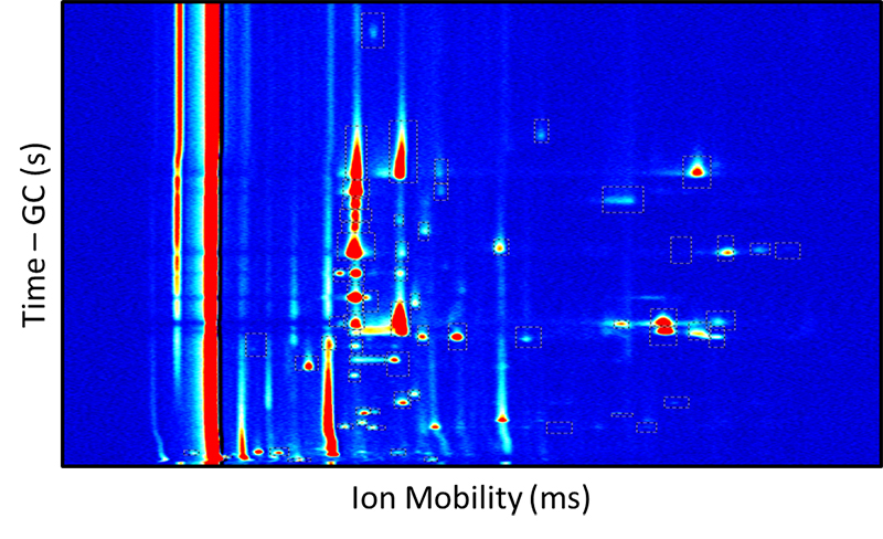
Figure 1. A somewhat typical GC/IMS analytical run showing relatively complex peak shapes compared to infrared spectroscopy.
With the introduction of the much more rapid ultra-high-performance liquid chromatography (UPLC® or UHPLC) systems, much effort was spent in increasing the speed at which the attached spectrometers were capable of scanning. This was so that sufficient data points could be obtained to properly define each peak, since analytes were eluting off the columns an order of magnitude faster, delivering much narrower, more intense peaks.
It is often the case that a system being studied is changing as it is being measured and this dynamic change is what you are studying. Clearly the time available for each independent measurement is constrained by the rate at which the system is changing, so it may not be possible to acquire many scans for each time point in order to achieve excellent signal-to-noise ratios.
A review by Engels and co-workers sums up some of the issues which lead to a demand for spectroscopic data pre-processing to remove unwanted artefacts in data sets under the headings of noise, baseline offset and slope light scatter temporal and spectral misalignment, normalisation, scaling and element-wise transformations, supervised pre-processing methods and finally artefacts in hyphenated techniques.1 This is an excellent starting point if you wish to go deeper into the subject than this column’s space allows. The authors acknowledge how extremely difficult it can be to determine which method or pre-processing methods can successfully be applied. It is important to take into account the specific data set characteristics emphasising that the identification of which artefacts are present among which properties of the spectroscopic data is of considerable importance that cannot be ignored in this choice of pre-processing strategies.
Approaches to spectroscopic data pre-processing: or “my boss told me to do it” syndrome
In some laboratories there are preferences for carrying out certain types of pre-processing as standard, and this includes standard ordering of the pre-processing steps. These have often been handed down over the years and the original reasons for these workflows are no longer known by the current laboratory staff.
Jan Gerretzen and co-workers at the University of Nijmegen working under the Dutch COAST initiative carried out some work to try and eliminate the “black magic” around the selection of the data pre-processing steps and the order in which they should be carried out. They adopted a systematic Design of Experiments approach to varying baseline, scatter, smoothing and scaling pre-processing steps for reference data sets in Latex monitoring (quantifying butyl acrylate and styrene) as well as corn data sets for their moisture content.2 In a separate report the approach was tested on data from a near infrared (NIR) spectrometer monitoring NaOH, NaOCl and Na2CO3 concentrations in a waste treatment system of a chlorine gas (Cl2) production facility. The gaseous waste effluent of this facility contains chlorine, which is removed by a caustic scrubber where the waste gases are led through a solution containing NaOH.3
Selection of pre-processing strategies
Quite often text books or spectroscopic data processing packages will describe the effect of individual pre-processing algorithms. However, there is little support around the consequences of applying multiple pre-processing steps during data analysis. Even the order that the pre-processing steps are applied can have a drastic effect on the quality of the analysis, let alone how the parameterisation of each step impacts subsequent steps or the final result.
Table 1 shows an experimental design used in this approach. A full factorial design was selected to evaluate the influence of each pre-processing step. The response variable measuring the model improvements from the pre-processing steps was the root-mean-square error of prediction figures.
Table 1. Data preprocessing Design of Experiments derived from Reference 1.
Experiment | Baseline | Scatter | Smoothing | Scaling |
1 | Yes | Yes | Yes | Yes |
2 | Yes | Yes | Yes | No |
3 | Yes | Yes | No | Yes |
4 | Yes | Yes | No | No |
5 | Yes | No | Yes | Yes |
6 | Yes | No | Yes | No |
7 | Yes | No | No | Yes |
8 | Yes | No | No | No |
9 | No | Yes | Yes | Yes |
10 | No | Yes | Yes | No |
11 | No | Yes | No | Yes |
12 | No | Yes | No | No |
13 | No | No | Yes | Yes |
14 | No | No | Yes | No |
15 | No | No | No | Yes |
16 | No | No | No | No |
Figure 2 shows how close the rapid Design of Experiments approach came to determining the best sequence and parameterisation of various pre-processing strategies, compared to identifying the absolute best strategy determined by Brute Force number crunching of every possible variable (over 5000 solutions required to be calculated).
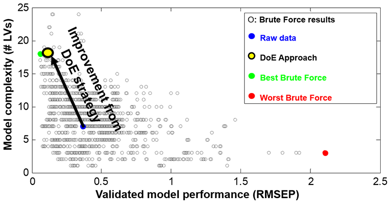
Figure 2. Successful application of a Design of Experiments approach to spectroscopic data pre-processing for model optimisation (data taken from the work reported in Reference 3).
Most authors highlight the fact that their work can really only be deemed applicable to the types of data and particular types of samples they are analysing. In Reference 1, the application of variable selection and data pre-processing were only observed to improve the model performance when they were carried out simultaneously2 and the conclusion was that although the specific “best-case” data pre-processing solutions were found, the more general applicability of this work was in defining a successful generic approach to scientifically decide on the best spectroscopic data pre-processing methodology to use.
Peter Lasch looked at spectral pre-processing for infrared and Raman spectroscopic techniques used in the field of biomedical vibrational spectroscopy and microspectroscopic imaging.4 Here techniques including cleaning the datasets (outlier detection), normalisation, filtering, detrending, transformations like ATR correction and “feature” selection are discussed. The article contains some interesting explanatory graphics and longer discussions on water vapour correction, different strategies for normalisation, baseline correction and data filtering for noise removal or spectral resolution enhancement (use of derivative filters). Raman-specific spectroscopic data pre-processing is also addressed, covering topics such as the removal of cosmic ray artefacts and fluorescence background signals. The author acknowledges that a combination of pre-processing steps is usually required to obtain the best results and bemoans the sparsity of systematic investigations in which the effectiveness of different ways of applying pre-processing workflows to the specific needs of subsequent quantitative or classification analytical procedures is investigated. The author acknowledges that it is one of the main data analysis tasks to adapt and optimise these workflows, but this is still more an art rather than a science!
Data smoothing
Often used to reduce random noise where further data accumulation is not possible. Depending on the data set data smoothing can damage the data set leading to distorted picture of the results. Some typical data smoothing methods include Moving Average across a number of data points, the number of points averaged is adjustable and Savitsky–Golay smoothing which fits a polynomial to segment of the data set. In Savitsky–Golay smoothing the order of the polynomial can be changed (first-order = Moving Average) as well as the range of data to be fitted.
ATR correction
Correction of mid-IR spectra sampled using the Attenuated Total Reflectance (ATR) technique for the penetration depth dependence related to the frequency in the spectrum. It does not attempt to correct for the refractive index differences between the sample and the crystal that can lead to “derivative-like” spectra.
Multiplicative Scatter Correction (MSC)
Rinnan and co-workers took a critical look at a range of pre-processing methods in NIR spectroscopy chemometric modelling including a group of scatter-corrective pre-processing methods includes Multiplicative Scatter Correction using a reference data sets. They also looked at how different pre-processing methodologies impacted on the quality of prediction results for six different spectrometers using filter, dispersive and Fourier transform technologies. In whichever combination they applied pre-processing they could only achieve at best a 25 % improvement in the prediction error—and the concluded with a warning about the risks associated with incorrectly setting the parameters for the window size or smoothing functions.5
Derivative filters
Quite a popular pre-processing strategy to enhance the resolution of complex spectra assisting in identifying overlapping peaks and also assists in minimising the influence of baseline effects. For instruments that acquire signals in the time domain such as Fourier transform infrared spectrometers several techniques exist to apply filters to enhance resolution and reduce noise in the time domain before the data is transformed to the frequency domain.
Conclusion
I think it is clear that we are often constrained from measuring the ideal spectra for our tasks and that data pre-processing can eliminate or mitigate some of the problems arising from having to handle sub-optimal measurements. However, it is also clear that these pre-processing steps need to be carried out with our eyes wide open and after giving the problem some thought. The computing power now commonly available allows us to also use the Design of Experiments approach to find the best pre-processing strategy for our specific data sets—and that this pre-processing strategy needs to be re-assessed for each individual problem and not blindly copied across from one spectroscopic field to another.
References
- J. Engel, J. Gerretzen, E. Szyman´ska, J.J. Jansen, G. Downey, L. Blanchet and L.M.C. Buydens, Trends Anal. Chem. 50, 96–106 (2013). https://doi.org/10.1016/j.trac.2013.04.015
- J. Gerretzen, E. Szyman´ska, J. Bart, A.N. Davies, H.-J. van Manen, E.R. van den Heuvel, J.J. Jansen and L.M.C. Buydens, Anal. Chim. Acta 938, 44e52 (2016). https://doi.org/10.1016/j.aca.2016.08.022
- J. Gerretzen, E. Szyman´ska, J.J. Jansen, J. Bart, H.-J. van Manen, E.R. van den Heuvel and L.M.C. Buydens, Anal. Chem. 87, 1209612103 (2015). https://doi.org/10.1021/acs.analchem.5b02832
- P. Lasch, Chemometr. Intell. Lab. Syst. 117, 100–114 (2012) https://doi.org/10.1016/j.chemolab.2012.03.011
- Å. Rinnan, F. van den Berg and S.B. Engelsen, Trends Anal. Chem. 28(10), 1201–1222 (2009). https://doi.org/10.1016/j.trac.2009.07.007