Carolina S. Silva,a,* Maria Fernanda Pimentel,a José Manuel Amigo,b Carmen Garcia-Ruizc and Fernando Ortega-Ojedac
aDepartment of Chemical Engineering, Federal University of Pernambuco, Av. Prof. Moraes Rego, 1235 – Cidade Universitária, Recife, Brazil
bDepartment of Food Science, University of Copenhagen, Rolighedsvej 30 - Frederiksberg C, Copenhagen, Denmark. E-mail: [email protected]
cDepartment of Analytical Chemistry, Physical Chemistry and Chemical Engineering and University Institute of Research in Police Sciences (IUICP), University of Alcalá, Ctra. Madrid-Barcelona Km. 33.6, 28871 Alcalá de Henares (Madrid), Spain
Introduction
In the forensic document examination field, document dating is one major challenge that still lacks validated methodologies. The variety of inks and papers, combined with different storage conditions, poses a complex problem when an estimation of age is needed. Although paper samples are mainly composed of cellulose, their chemical composition changes according to the manufacturing process and the raw materials. When paper samples start degrading, differences in chemical profile can be identified. However, differences in the initial composition must be considered to avoid misinterpretation.
Spectroscopic techniques such as mid-infrared are increasingly important in forensics.1 One of the main reasons is the non-destructive and non-invasive nature of the analysis, which is able to provide chemical information whilst maintaining the integrity of the samples.
The aim of this work is to evaluate paper variability in document dating. To do this, mid-infrared spectroscopy, together with chemometric techniques, were used to estimate the document age of papers of different natures; for more detailed information, see Reference 2.
Chemometrics
Mid-infrared spectroscopy has the great advantage of providing a large amount of spectral information over a wide wavelength range. The disadvantage is that the spectral information is often redundant and affected by spectral artefacts. Therefore, multivariate techniques of analysis (a.k.a. chemometrics) are needed to extract useful chemical knowledge.
Principal component analysis (PCA) is probably the best-known chemometric technique. It is an exploratory technique of analysis that uses maximum variance to describe the dataset in a new space with reduced dimensionality. In contrast to PCA, partial least squares (PLS) is a supervised technique that aims at building a mathematical model based on spectral features to predict a parameter of interest, in this case, the age of a given document. To do this, a set of samples with a known age (Training set) is employed to establish a mathematical relationship between the spectra and the age, maximising the covariance between them. Extensions of PLS, such as sparse partial least squares (sPLS), can be employed as variable selection methods. In this case, sPLS imposes a penalty term to uninformative coefficients to have zero value, reducing noise and attenuating the influence of correlated or unrelated variables present in the spectral profile.
As mentioned above, physical phenomena can cause variation in the dataset that is not relevant to the study (such as noise, baseline etc.) and these can mask the information of interest. Spectral preprocessing techniques can be used to correct or minimise the effect of these undesired phenomena and provide a reliable analysis. In other cases, chemical interferences can be the cause of such problems. Therefore, more dedicated methods are needed to correct those contributions. Orthogonal signal correction (OSC) and generalised least squares weighting (GLSW) are examples of these techniques.
While OSC subtracts the variability of spectral data that is orthogonal to the age, GLSW applies a filter matrix to down-weight the interferent contribution. Further information can be found elsewhere.3,4 To evaluate model performance, validation and prediction sets were investigated, providing information about the model’s ability to predict unknown samples.
Materials and methods
Reports from 15 different years between 1985 and 2012 were provided by the Spanish General Commissary of Scientific Police (Madrid, Spain). For each year, five reports containing an average of five sheets each were analysed with mid-infrared spectroscopy. Eight spectra were acquired per sheet. A Nicolet iS10 spectrometer (ThermoFisher Scientific, MA, USA) was employed for spectral acquisition with the Smart iTR diamond attenuated total reflectance accessory. The spectral range investigated was 4000–650 cm–1, with resolution of 4 cm–1 and 32 scans per spectrum.
The samples described above were used to build two different datasets with different criteria of selection to compose the Training and the Prediction sets. The Prediction set for both datasets was, in turn, split into so-called Report Prediction and Sheet Prediction sets. In dataset-PCA, PCA was performed to select one whole report from each year to compose the Report Prediction set, guaranteeing that all plausible variability is included in the model and no extrapolations were made. In contrast to the statistical philosophy, but tuned for the forensic application, the dataset-RANDOM was built by randomly choosing a whole report from each year to compose the Report Prediction set. For both datasets, the Sheet Prediction set was built by randomly choosing one sheet from the remaining reports.
PLS models were built and compared, employing different preprocessing techniques to attenuate differences among documents from the same year. All chemometric analysis were made using the PLS_Toolbox (Eigenvector Research Inc., USA) running on Matlab (The Mathworks, MA, USA). The sPLS algorithm was used as described in Reference 5.
Results and discussion
Spectral profiles of papers (Figure 1) showed the important cellulose-related bands, such as the characteristic O–H bond vibration at 3400 cm–1, absorptions at 1025 cm–1, 1160 cm–1, 1315 cm–1 and 2890 cm–1, related to different C–H, C–OH, C–CH2, C–O–C vibrations, respectively. These contributions are common to all paper samples, regardless of their age. Calcium carbonate (712 cm–1 and 870 cm–1) and kaolinite (3690 cm–1 and 3620 cm–1) absorptions were also found; these compounds are usually employed as inorganic fillers. These contributions are not common to all paper samples, but vary according to the manufacturing process; papers from the same year can have different compositions of these inorganic fillers.
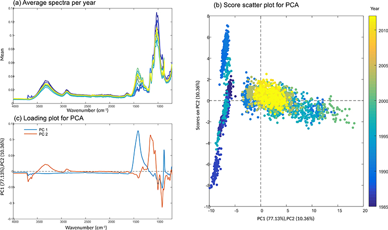
Figure 1. (a) Average spectra per year, (b) score and (c) loading plots of PCA.
This variability of paper composition poses a big challenge in document dating, because models to estimate paper age can be built based on the different chemical composition rather than differences due to the aging process. If the variability of samples is not considered in a proper manner, models can be optimal from a mathematical point of view but misleading as to the final aim. To reduce that variability, preprocessing techniques and variable selection were employed.
PCA shows the difference between the document types. According to Figure 1, it is possible to observe that samples from year 1990 show more than one cluster (see score scatter plot), indicating a different chemical composition. In the loading plot it is possible to observe that these differences are explained in PC1 by the inorganic fillers’ absorption bands.
After confirming the variability within samples from the same year, four PLS models with different preprocessing techniques and variable selection strategies were compared using the two datasets. Table 1 shows that results from dataset-RANDOM show higher prediction errors (root mean square error of prediction, RMSEP) for Report Prediction for all models, a trend that is repeated in the bias of the models. This is due the fact that some of the reports in the prediction set show high variability when compared to the training set.
Table 1. Results from the PLS models using different preprocessing techniques Model 1 [PLS model with standard normal variate (SNV), smoothing and mean-centring]; model 2 (PLS model with SNV, smoothing, OSC and mean-centring); model 3 (PLS model with SNV, smoothing GLSW and mean-centring); and model 4 (sPLS model with SNV, smoothing and mean-centring).
|
| Dataset-PCA | Dataset-RANDOM | |||||||
Model | 1 | 2 | 3 | 4 | 1 | 2 | 3 | 4 | ||
LV | 4 | 1 | 2 | 5 | 4 | 1 | 3 | 5 | ||
Training set | RMSECV | 4.7 | 4.5 | 4.6 | 4.5 | 4.4 | 4.5 | 4.2 | 4.3 | |
R2cv | 0.83 | 0.85 | 0.86 | 0.88 | 0.74 | 0.74 | 0.76 | 0.73 | ||
biascv | 0.04 | 0.02 | 0.01 | –0.06 | 0.01 | 0.04 | –0.00 | 0.87 | ||
Prediction set | Report | RMSEP | 3.8 | 4.0 | 3.6 | 4.0 | 5.1 | 4.3 | 5.0 | 4.7 |
R2pred | 0.90 | 0.89 | 0.91 | 0.88 | 0.74 | 0.80 | 0.75 | 0.86 | ||
bias | 0.35 | 0.32 | 0.22 | 0.15 | 2.11 | 1.46 | 1.95 | 0.64 | ||
Sheet | RMSEP | 4.3 | 3.7 | 4.2 | 4.5 | 4.0 | 3.6 | 3.7 | 4.3 | |
R2pred | 0.86 | 0.90 | 0.87 | 0.85 | 0.78 | 0.82 | 0.82 | 0.87 | ||
bias | 0.05 | 0.24 | 0.07 | 0.00 | 0.44 | 0.22 | 0.34 | 0.97 | ||
LV: number of latent variables; RMSECV: root mean square error of cross validation; RMSEP: root mean square error of prediction
From Table 1 is clear that the preprocessing filters decrease the model complexity [number of latent variables (LV)]. When OSC and GLSW are applied, a significant, but not relevant, amount of variance is removed from the dataset, leading to its simplification.
Comparing all strategies, OSC (model 2) showed potential in model building. With one LV, the model decreased the prediction error when compared to the other models and showed more stability regarding Report Prediction error for the two datasets built. In addition, the most important variables in model 2 (Figure 2) to estimate document age were 1412 cm–1 and 914 cm–1. According to the literature, those two bands reflect changes in cellulose crystallinity during the degradation process, while other research has assigned the 1410 cm–1 absorption to the filler compounds. Although the spectral region appears to have an ambiguous interpretation, it is important to mention that the obtained values of approximately four years for RMSECV/RMSEP are adequate for the proposed application and the complexity of the samples.
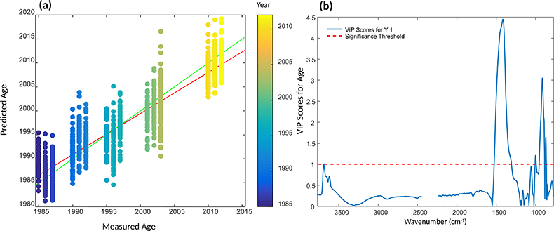
Figure 2. Results for the PLS regression model 2 (applying OSC filter with one component): (a) regression plot and (b) VIP scores for model 2.
Conclusion
The most important point of this study was to open a discussion about the implementation of spectroscopic and chemometric techniques in complex contexts such as forensics, especially regarding document aging. This is extremely important because it is not known if the degradation processes are similar for samples with different chemical compositions. Nonetheless, this study shows the potential of infrared spectroscopy and chemometrics to assess document age. It also provides the prospect of implementing advanced analytical methodologies in scientific police laboratories.
Acknowledgements
The authors would like to acknowledge the Spanish General Commissary of Scientific Police (Documentoscopy section, Spain) for providing the analysed documents. Also, the funding agencies INCTAA (Processes no.: CNPq 573894/2008-6; FAPESP 2008/57808-1), NUQAAPE – FACEPE (APQ-0346-1.06/14), Núcleo de Estudos em Química Forense – NEQUIFOR (CAPES AUXPE 3509/2014, Edital PROFORENSE 2014), CNPq (PVE/CNPq, process no: 400264/2014-5), FACEPE and CAPES (PDSE scholarship process number BEX 7712/15-4), are acknowledged.
References
- C.K. Muro, K.C. Doty, J. Bueno, L. Halámková and I.K. Lednev, “Vibrational spectroscopy?: recent developments to revolutionize forensic science”, Anal. Chem. 87, 306–327 (2015). doi: https://doi.org/10.1021/ac504068a
- C.S. Silva, M.F. Pimentel, J.M. Amigo, C. García-Ruiz and F. Ortega-Ojeda, “Chemometric approaches for document dating: handling paper variability”, Anal. Chim. Acta 1031, 28–37 (2018). doi: https://doi.org/10.1016/j.aca.2018.06.031
- S. Wold, H. Antti, F. Lindgren and J. Öhman, “Orthogonal signal correction of near-infrared spectra”, Chemometr. Intell. Lab. Syst. 44, 175–185 (1998). doi: https://doi.org/10.1016/S0169-7439(98)00109-9
- N.B. Gallagher, “Detection, classification, and quantification in hyperspectral images using classical least squares models”, in Techniques and Applications of Hyperspectral Image Analysis, Ed by H. Grahn and P. Geladi. John Wiley & Sons Ltd, pp. 181–202 (2007). doi: https://doi.org/10.1002/9780470010884.ch8
- R. Calvini, A. Ulrici and J.M. Amigo, “Practical comparison of sparse methods for classification of Arabica and Robusta coffee species using near infrared hyperspectral imaging”, Chemometr. Intell. Lab. Syst. 146, 503–511 (2015). doi: https://doi.org/10.1016/j.chemolab.2015.07.010