A.M.C. Davies
Norwich Near Infrared Consultancy, 10 Aspen Way, Cringleford, Norwich NR4 6UA, UK. E-mail: [email protected]
Introduction
Yes, this really is the last TD Column by me [but the other TD (Antony N.) will be continuing]!
I did think about recounting the story of the birth of the TD Column but instead I am going to concentrate on another story which started some years before the column and is still not completed. I vaguely introduced it in the last column:1 quantitative analysis from NIR data using the CARNAC procedure. The story really starts a long, long time ago; around 3500 years. At this time my Neolithic/Celtic ancestors helped to construct what is believed (by some) to be a gigantic lunar observatory at what is now Carnac, Brittany, France. It has been demonstrated that the stone structures could be used to follow and predict the motion of the moon. One of the striking features of the area is the “alignments” at Carnac, which are 12 rows of large stones that extend for five kilometres. These might have been used to extrapolate observations of the moon during periods when unfavourable weather prevented direct observations. I learned of Carnac from a New Scientist article in 19722 shortly before holidaying in that area and seeing them for real; an experience I have never forgotten.
CARNAC
I began working in NIR spectroscopy in 1980 at the Institute of Food Research (IFR) in Norwich, UK. One of the data sets for which I had been asked to make a calibration was proving very difficult. When one of the analytes was plotted against another, the plot contained clusters of samples with quite large gaps with no samples. In 1983 I attended a conference in Aberdeen, UK, and during the eight-hour train journey back to Norwich I had time to think if I had learned anything that would help solve the problem. I have no idea why, but I suddenly saw the data clusters as stones in the Carnac alignments and thought that if I could assign an unknown sample to the correct cluster (or stone) then I would be able to assign the analytical values associated with that stone (or cluster) to the unknown sample. So rather than try to form calibration models, the alternative problem was to search a database of analysed samples to find very similar samples so that their analyte values could be assigned to the unknown sample. We had begun work on writing programs to make the required calculations before I realised that there was a serious problem. Spectra would be dominated by the major ingredient (or more accurately specified as the major absorber) and so it could only be expected to provide useful results for this single analyte. However, the proposal was saved by the additional idea that we needed to emphasise the absorptions of the intended analyte. We would thus need to reconstruct the database by multiplying each spectrum by a modification vector which would be different for each analyte. The first method for determining this modification vector was the weights obtained from a traditional multiple linear regression (MLR) regression which has been used in most of the reported work, but other sources (principal component analysis and pure spectra of the analyte) have also worked.

In the initial development period (1983–1987) computers were slow and very limited, so an additional problem would have been that spectral databases (700 variables in a spectrum) would have been much too large for the available computers. However, I had met Professor Fred McClure (who worked at North Carolina State University, USA) at the first International Diffuse Reflectance Conference in 1982 and we were collaborating on applications of his idea to compress spectral data by Fourier Transformation (FT). So this was not a problem for us and we used the first 50 a and b coefficients from FT to replace 700 (or more) wavelength variables. Fred had shared his suite of FORTRAN programs for NIR analysis and so the first version of CARNAC was a modified version of one of these programs. Fred also had a database of coffee spectra with analytical values for chlorogenic acid and caffeine and I choose to start with caffeine because this is a minor constituent of coffee (1–4%). While working in Fred’s lab in Raleigh, NC, USA, in 1985 we achieved the first successful run of the program on 4th July. There were many fireworks later in the day (did the news get out?)!
After this initial success, we worked on a few more databases, I talked about CARNAC at the 1986 Chambersburg Conference and we presented a poster at the FT conference in Vienna which became the first publication.3 In 1987 I was made redundant by IFR and joined Oxford Analytical Instruments where there was little time to spend on academic research and in July 1989 I became an independent consultant with even less time for research. That was almost the end of the CARNAC development.
CARNAC was saved by Fred McClure in 1997 when he told me that John Shenk had developed a new method (LOCAL) which sound a little like CARNAC and urged me to have another attempt to develop it. By this time our orginal programs had been made obsolete by the “Windows” take-over of small computer systems, so Tom Fearn agreed to collaborate with me to write a new set of programs in MATLAB™ and include wavelets as an alternative compression technique. However, it did take some time to get this underway and it was not until 2002 that we had a working suite of programs for CARNAC-D (the D is for “deux”) and 20064 before we published a description of the re-birth of the idea. Progress has been very slow in recent years (we have had variety of problems), but we did some very encouraging work with Ana Garrido-Varo and her team at Córdoba, Spain, when they compared the performance of several methods on some very large databases of feed ingredients. CARNAC produced the best results.5 I am going to make an extra effort to publish our promised next paper giving results for three databases in the near future!
How does it work?
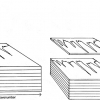
Although CARNAC operates without supervision, it is convenient to consider it in two stages, as indicated in Figures 2 and 3.


In stage 1 the spectra in the database are compressed, SMLR run and a modification vector selected from the SMLR. This vector is then used to modify all the spectra in the database. The spectrum of the unknown sample is compressed and then multiplied by the modification vector. This modified spectrum is then compared to each modified spectrum in the database and a similarity index is calculated. The output from this stage is thus an array of similarity values and y (analyte values). In stage 2 the output array is analysed for each spectrum to find those members which are very similar to the spectrum of the unknown sample. The weighted mean of the y values of these samples is then calculated as the predicted y value of the unknown sample. There are eight critical parameters that can be changed to optimise the results. This can be achieved (with experience!) fairly quickly because the program takes less than 5 s to process 100 unknowns with a database of 500 spectra. The program will sometimes fail to find any very similar samples and cannot give a result. Some critics do not like this, but I think it is a strength of the method that it works this way and does not provide unreliable results.
Why it works
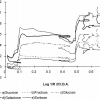
Figure 4 demonstrates that the train inspiration really works.

The plot of similarity against analyte concentration is even better than the one I sketched on my train ticket. The black dots are samples with low similarity to the test sample; most were excluded by the horizontal line of minimum similarity while the remaining black dots were excluded because their similarity was considerably less than the selected (red) samples. One red dot has been excluded because of its analyte distance from the other selected results. The solid blue line is the predicted concentration of the analyte in the test sample (39.5) while the dashed green line is the actual result by analysis (40.6).
Is there a future for CARNAC?
I hope so! It has taken a very long time to develop, but this was partially inevitable because the method required scanning NIR spectrometers, large databases of scanned and chemically analysed samples and large and fast computers in quality control laboratories. None of these were generally available in 1983 but now they are. The other main difficulty has been finding the time for non-funded developments in our busy schedules! Now that the technical requirements are in-place we are determined to find the time to complete the project.
What are the prospects for chemometrics?
I started writing these columns in Spectroscopy World6 (1989–1992) and then in Spectroscopy Europe (1992–2014) which has been a very good period to have been writing about chemometrics. I was very excited by chemometrics in 1989, it is still exciting but the pace of development has slowed down and become technically more challenging (I am 25 years older and have lost many neurons!). There are new chemometric tools that we know we need. I think improvements in handling hyperspectral data is an obvious one but the more exciting ones (not yet conceived or developed) currently do not have any application—I look forward to reading about them when they arrive!
Acknowledgements
Before I finish I want to acknowledge some people without whom this column might not have got started; it definitely would not have continued for so long. The first has to be Ian Michael because he invited me to do it and has always been very supportive and helpful. Thanks Ian, it has been fun! Next (and only just second) is Tom Fearn. Without Tom to explain things until I “got them”, write lots of MATLAB™ code, gently tell me when I was writing nonsense, let me borrow his figures and ideas from “The Chemometric Space” (in NIR news) etc. etc. … Thanks Tom.
We all need to thank Svante Wold for coining the word, chemometrics. The “folk law” is that he invented it for a funding application; I once had a very pleasant supper with him and asked him “was it true?” “Yes it was”, but “Was it successful?”, “Yes”. I was very pleased for him.
Finally, I would like to thank contributors, readers and friends who have encouraged me. I would like to quote Douglas Adams “So Long and Thanks for all the Fish”7 but I’m not planning on leaving the earth just yet!
Best wishes

References
- A.M.C. Davies, “The last furlong (5). Classification and identity testing”, Spectrosc. Europe 26(4), 24 (2014). http://bit.ly/1°OAnef
- S. Mitton, New Scientist 13 April, 60 (1972).
- A.M.C. Davies, H.V. Britcher, J.G. Franklin, S.M. Ring, A. Grant and W.F. McClure, “The application of Fourier-transformed NIR spectra to quantitative analysis by comparison of similarity indices (CARNAC)”, Mikrochim. Acta (Wien) I, 61–64 (1988). doi: http://dx.doi.org/10.1007/BF01205839
- A.M.C. Davies and T. Fearn, “Quantitative analysis via NIR databases: Comparison Analysis using Restructured Near infrared And Constituent data-Deux (CARNAC-D)”, J. Near Infrared Spectrosc. 14(6), 403 (2006). doi: http://dx.doi.org/10.1255/jnirs.712
- D. Pérez-Marín, A. Garrido-Varo, J.E. Guerrero, T. Fearn and A.M.C. Davies, “Advanced non-linear approaches for predicting the ingredient composition in compound feedingstuffs by near infrared reflection spectroscopy”, Appl. Spectrosc. 62(5), 536 (2008). doi: http://dx.doi.org/10.1366/000370208784344389
- T. Davies, “Strings and stripes”, Spectrosc. World 1(1), 30 (1989).
- D. Adams, So Long and Thanks for all the Fish. Pan Books Ltd (1984).