A.M.C. Daviesa and Tom Fearnb
aNorwich Near Infrared Consultancy, 75 Intwood Road, Cringleford, Norwich NR4 6AA, UK. E-mail: [email protected]
bDepartment of Statistical Science, University College London, Gower Street, London WC1E 6BT, UK. E-mail: [email protected]
Introduction
In our previous column1 we introduced some distance statistics that have been used for comparing spectra. These calculations provide univariate answers from multivariate data in a single step. This may be adequate for some problems but often we need to employ some multivariate mathematics before the reduction to a univariate answer.
This column is an introduction to the first method, which was invented long before chemometrics by R.A. Fisher; some seventy years ago! Canonical Variates Analysis (CVA)2 has been one of my favourite examples of chemometrics because it often requires the use of a compression technique (PCA or FFT for example) before it can be applied and I think it helps students to understand the need to know the essential properties of the different tools in the chemometric toolbox.
Tony Davies
Groups
In multivariate analysis of spectroscopic data it is very unusual to compare an unknown with a single spectrum of a known sample. It is normal to collect spectra from several examples of the same sample into a group and compare the unknown spectrum with the group. This is because when we make measurements there will always be some variation between different examples and we need to have information about the variability of the group. In fact instrument noise ensures that spectra of the same example measured on the same instrument will have some variability.
Canonical variate analysis
The CVA technique has similarities with PCA in that the multivariate data is submitted to the program which computes new variables and values (scores) for each sample and each of the new variables. In PCA the new variables are principal components, while in CVA they are canonical variates. Where they differ is in how the new variables are selected. PCA is not given any information about groups and group membership, it is just required to compute new variables to maximise the variability of the scores for the whole data set. CVA is given information about groups and group membership and the requirement is that new variables will minimise the within-group variation while maximising the between-group variation. As shown in Figure 1(a) and (b), the within-group variance, Wg, is a pooled result from all the groups being considered. When the groups have different variability, as in Figure 1, Wg is a compromise, but the approach often works well in spite of this.

Figure 1. Calculation of the pooled within-group variance and the between-group variance for CVA with three groups of samples.
Bg is the between group variance and the criterion to be maximised is the ratio Bg/Wg.
To apply CVA, the number of input variables must be less than (in reality considerably less than) the number of samples. This presents a difficulty with spectroscopic data that usually has a large number of variables (wavelengths or wavenumbers). The possible solutions are to discard the majority of datapoints or (as mentioned earlier) to use some form of compression to retain most of the information in the original data but compressed into fewer variables. The most obvious of these is PCA.
One difference between PCA and CVA is that the transformation from original variables to scores in PCA is a simple rotation in which the axes remain mutually orthogonal. In CVA the angles between the axes and the scaling of the axes changes so that the elliptical shape describing within-group variability (and corresponding to Wg) becomes a circular or spherical shape. In consequence, measuring using Euclidean distances in CV-space corresponds to using Mahalanobis distance in the original spectral space, and classification using the CVA approach is equivalent to classification using Mahalanobis distance (see our frequently referenced book3 for a description of Mahalanobis distance).
Examples
a) Two groups
With two groups we need to find only one CV. The example was mentioned in the first “Chemometric Column” in Spectroscopy World4 and again in an early “Tony Davies Column”.5 It involves the separation of regular and decaffeinated instant coffee samples from their NIR spectra. The spectra, Figure 2(a), show no separation. The spectra contained 700 datapoints and at that time our best PCA program would accept only 50 variables. One way to utilise this program was to reduce the number of wavelength variables by averaging successive 14 data points leaving 50 variables so that these could be used as the input data. Then the first ten PCs were used as the input data to a CVA program. The result is shown in Figure 2(b). An alternative method was to use Fourier transformation (FT) to compress the data to 25 pairs of Fourier coefficients which were used as the input data to the PCA program. The result obtained from the CVA using the first ten PCs is shown Figure 2(c). Nowadays, PCA programs accept much larger numbers of input variables but at the time it was a demonstration of the value of compression by FT and also the value of using chemometrics tools for their designed application.
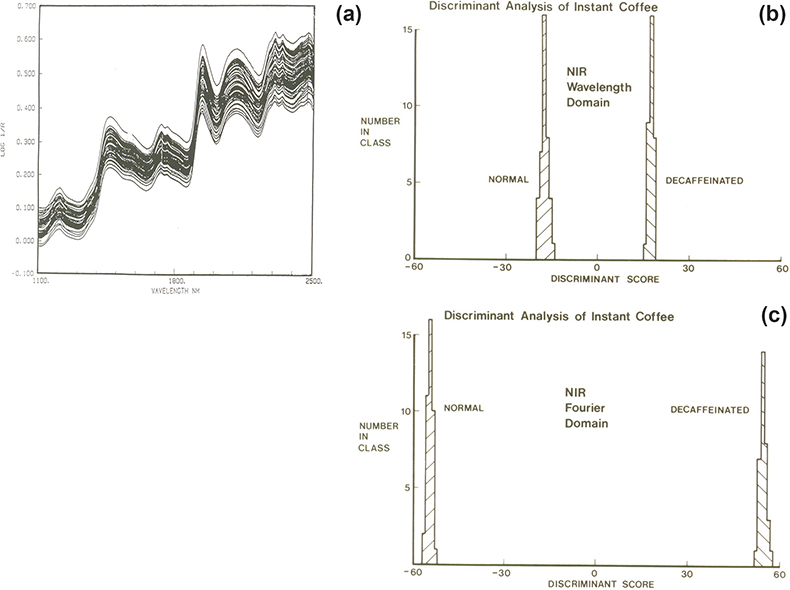
Figure 2. (a) NIR spectra of regular and decaffeinated instant coffee, (b) CVA result using the 50 point wavelength domain data, (c) CVA result using 50 point (25 × 2) FT data.
b) Several groups
This example is from some later work to attempt to identify the botanical origin of honey samples from their NIR spectra.6 Second derivative spectra were used as the input data to a PCA program and the first ten or first fifteen PCs were used as the input data to a CVA program. This work was very much a preliminary study because there were very few samples available. The work was validated using cross-validation leaving out one sample at a time and recalculating the PCs as well as the CVs. Although the best separations used three CVs it is easier to look at just the first two. Figure 3(a) shows the PCA result for one particular sample removed and Figure 3(b) shows the CVA result obtained from this data. These graphs are an excellent example for demonstrating the superior power of CVA compared to PCA for separating similar samples. Many people use PCA for identification; it does work in many cases but it only works by accident because the variability in the data is related to the differences between samples. PCA is an “unsupervised method” it cannot make use of the information about group membership to improve the separation.
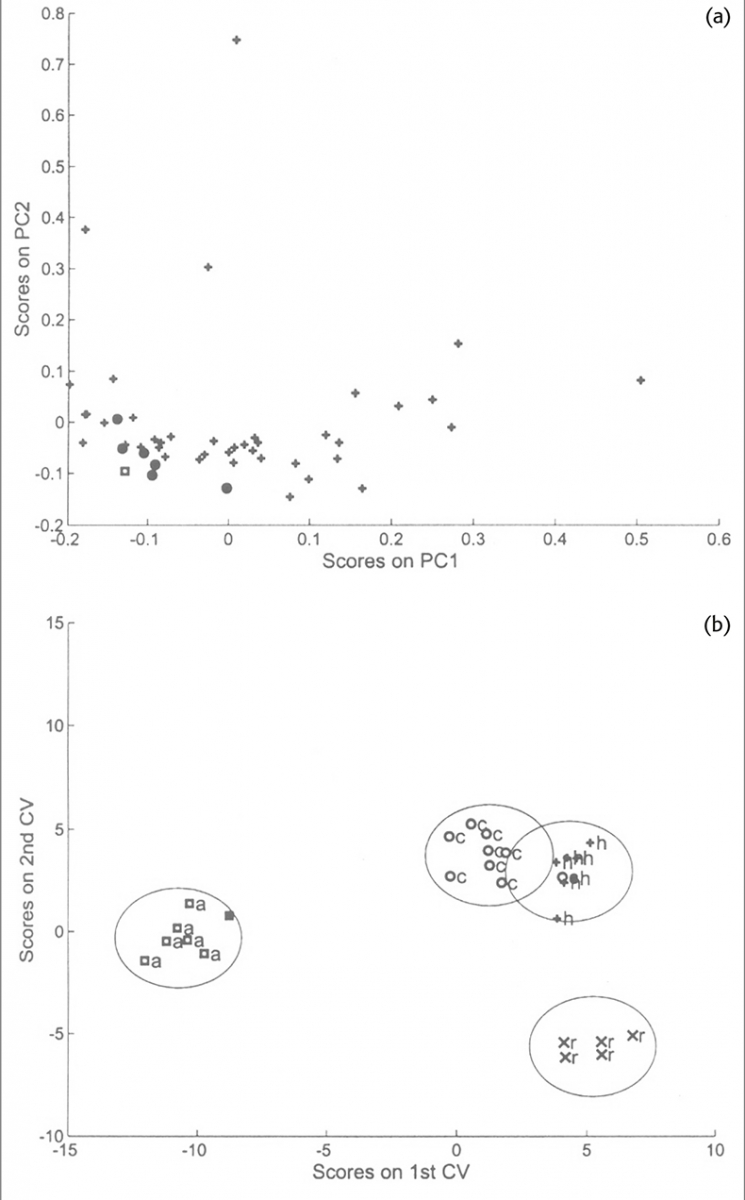
Figure 3. (a) Scores plot of the first two PCs indicating the position of the acacia samples (circles) in the distribution of 48 honey samples. The square symbol indicates the position of an acacia sample which was excluded from the PCA. (b) Plot of the first two CVs. The four groups of honey are indicated by the 0.95 confidence boundaries around each group. The square symbol indicates the computed position of the acacia sample omitted from the analysis.
Coming soon
In our next column we will discuss the more recently developed method of SIMCA and discuss the other factors which must be taken into consideration before discrimination decisions can be made.
References
- A.M.C. Davies and T. Fearn, Spectroscopy Europe 20(2), 15 (2008).
- R.A. Fisher, Ann. Eugen. 7, 179–188 (1936). https://doi.org/10.1111/j.1469-1809.1936.tb02137.x
- T. Næs, T. Isaksson, T. Fearn and T. Davies, A User-Friendly Guide to Multivariate Calibration and Classification. NIR Publications, Chichester (2002).
- A.M.C. Davies, Spectroscopy World 1(1), 30 (1989).
- A.M.C. Davies, Spectroscopy Europe 5(6), 30 (1993).
- A.M.C. Davies, B. Radovic, T. Fearn and E. Anklam, J. Near Infrared Spectrosc. 10, 121–135 (2002). https://doi.org/10.1255/jnirs.329


