Determination of soil organic matter using visible-near infrared spectroscopy and machine learning

Full-Text PDF

Felipe Bachion de Santana,^a Sandro Keiichi Otani,^b André Marcelo de Souza^c and Ronei Jesus Poppi^d

^aInstitute of Chemistry, University of Campinas (UNICAMP), PO Box 6154, 13084-971 Campinas, SP, Brazil
^bInstitute of Chemistry, University of Campinas (UNICAMP), PO Box 6154, 13084-971 Campinas, SP, Brazil
^cBrazilian Agricultural Research Corporation (Embrapa Soils), 22460-000, Rio de Janeiro, RJ, Brazil
^dInstitute of Chemistry, University of Campinas (UNICAMP), PO Box 6154, 13084-971 Campinas, SP, Brazil. E-mail: [email protected]

Introduction

United Nations (UN) projections estimate that the world’s population will be around 9.6 billion by 2050. Current projections indicate that feeding such a huge population would require dramatically increasing (~70 %) overall food production by 2050. To achieve this goal, the agricultural productivity in developing countries such as Brazil would need to increase significantly in order to provide more productive, sustainable and inclusive food systems to fight poverty and hunger in this massive population. One of the most important factors required to accomplish this task is the understanding of soil fertility in order to manage it most effectively.

To achieve this, millions of soil analyses are performed every year around the world to increase crop yields. In Brazil, approximately 4 million soil fertility analyses are performed per year, and soil organic matter (SOM) is one of the main factors that support land management. However, the two main conventional methodologies to determine the SOM (Walkley–Black and dry-combustion) are time-consuming and expensive, and hence are not suitable for use on a large scale. Also, the Walkley–Black method is damaging to the environment, generating residues that require treatment, and, therefore, is not suitable for sustainable agricultural practices.¹

As an alternative to the traditional methods, visible-near infrared (vis-NIR) spectroscopy can provide fast, low-cost and accurate results for SOM analyses in an environmentally friendly way. Also, the methodology is non-destructive and does not require additional sample preparation. A comparison between the two methodologies is illustrated in Figure 1.

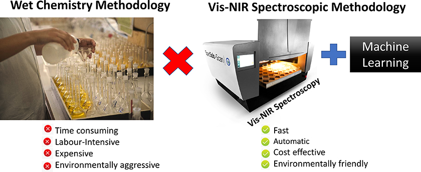
Figure 1. Comparison between the wet and vis-NIR spectroscopic methodology for SOM analysis.

However, vis-NIR spectra are composed of wide and superimposed bands and thus the application of this type of spectroscopy in SOM determinations requires the development of multivariate regression models capable of correlating these bands with the SOM reference values. Also, the soil matrices are very heterogeneous, complex and require a tremendous number of samples to create robust vis-NIR calibration models. Due to these problems, machine learning methods with high generalisation power have been employed in the development of the models. Among the machine learning methods that are suitable, we highlight the support vector machine (SVM).²

Support vector machine

Support vector machine is a kernel-based machine learning method proposed by Vladimir N. Vapnik, which uses implicit mapping of the input matrix (vis-NIR spectra) into a high-dimensional feature space defined by a specific kernel function; in this case the radial basis function (RBF):²

$$K\left( {{x_i},{x_j}} \right) = exp\left( { - \gamma {{\left\| {{x_i} - {x_j}} \right\|}^2}} \right),{\rm{ }}\gamma > 0$$

(1)

In the feature space, a linear hyperplane is built with the maximal margin between the support vectors of each class, and this hyperplane is set up to solve the initial separation problem. The SVM can also be extended to regression problems by adding and subtracting a positive k number in the y_i reference value, creating a positive (y_i + k) and negative class (y_i – k). In this situation, the optimal separation hyperplane will pass by the original values of y_i, because the best separation will be y_i + 0. As in linear regression models, the y prediction value can be estimated using a linear regression function:

y = w · K(x) + b

(2)

where w and b are the slope and offset of the regression line. The optimal w and b are obtained by minimising Equations 3 and 4.

Minimise: $${1 \over 2}\left\| w \right\| + C\;\mathop \sum \limits_{i = 1}^n \left( {{\xi _i} + \xi _i^*} \right)$$

(3)

Subject to: $$\left\{ {\matrix{ {{y_i} - w.K\left( {{x_i}} \right) - b\; \le \varepsilon + \;{\xi _i}} \cr {w.K\left( {{x_i}} \right) + b - {y_i}\; \le \;\varepsilon + \;{\xi _i}} \cr {{\xi _i},\xi _i^{\rm{*}} \ge 0} \cr } } \right\}$$

(4)

where ε is the sensitive parameter which represents the tolerated error and C is the cost parameter, which controls the influence of each individual support vector. The slack variables ζ_i and ζ_i^* are introduced to account for samples that do not lie in the ε-sensitive zone.³

During this process the combination of two parameters must be optimised, the cost parameter (C) already described and the RBF kernel parameter (γ). γ is the regularisation parameter of the RBF function, which controls the width of this function. In order to reduce the time required to find this optimum combination, Bayesian optimisation can be used. The Bayesian optimisation algorithm attempts to minimise the root mean square error of cross validation (RMSECV) in a specific domain for each parameter; in this case [10^–3 to 10³] for C and γ. The algorithm selects the combination of C and γ points that provides the greatest potential improvement of RMSECV.⁴ SVM modelling and Bayesian optimisation were implemented in Matlab R2016b with the Statistics and Machine Learning Toolbox 11.0.⁴

Materials and methods

In order to obtain a spectral library that represents the major producing regions of Brazil, 42,471 soil samples from several regions of Brazil were collected. The SOM reference analyses were based on the Walkley–Black method. These analyses were performed in collaboration with the IBRA Laboratory, Brazil, that holds a certification of proficiency from the Brazilian Agricultural Research Corporation (Embrapa Soils) and is accredited to ISO/IEC 17025:2005.

Before the vis-NIR spectra acquisition, the samples were oven dried at 40 °C for 48 hours, a rubber mallet was used to break the soil clusters and the granule size was controlled by a sieve (Ø < 2 mm). The spectra were obtained using a vis-NIR spectrometer customised for this determination, called SpecSoil-Scan (Speclab Holding S.A., Campinas - SP, Brazil). This instrument can analyse 40 soil samples per batch and the spectral range is 432–2448 nm, with a spectral resolution of 3.3 nm.

A principal component analysis (PCA) model was applied to the spectral data set to find outliers. Samples with high values of Hotelling T² and residuals in spectral data (Q-statistics) at a significance level of 5 % were considered outliers. The Hotelling T² is related to leverage, which measures the distance of the sample from the centre of the data and Q residuals represent the unmodelled vis-NIR spectra.⁵

Representative samples were selected for development and validation of the models, resulting in 28,314 samples for the calibration set and 14,157 for the validation set.

Results and discussion

The original vis-NIR spectra of all soil samples are shown in Figure 2a, where the mean spectrum is represented by the black line. The NIR spectra contains useful information related to the SOM, due to absorptions in the CC, C=C, CH, CN, NH and OH chemical bands. In the visible region, information on the SOM can be determined from absorption bands due to chromophores and darkness of the soil.⁶

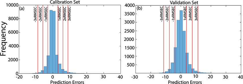
Figure 2. Original vis-NIR soil spectra (a) and preprocessed spectra (b).

To reduce baseline variation and spectral noise, the vis-NIR spectra were preprocessed by Savitzky–Golay smoothing and first derivative, with a window size of 11 points.⁷ The preprocessed spectra are shown in Figure 2b, where the major variations in the absorption bands at 400–600, 1100, 1400, 1800–2000 and 2200–2400 nm are highlighted, common to most soil samples.⁶

The three main absorptions bands are in the region of 500–650 nm, 1400 nm and 1900 nm. The absorptions at 500–650 nm can be associated with minerals that contain iron and the band at 1400 nm and 1900 nm can be associated with the OH group. The absorption band at 1100–1150 nm can be associated to aromatics and C–H stretch, and at 2200–2500 nm they are mainly due to vibrations involving metal–OH.⁶

The SVM model was built using the calibration samples and the choice of the optimal combination of C and γ values was performed as described above. To avoid overfitting in the regression model, the validation set was considered a set of unknown samples and these samples had no influence on the choice of C and γ parameters of the SVM model.

The scatter plots showing the reference versus predicted values by the SVM model are shown in Figure 3. Due to the high number of samples a colour bar containing the recurrence of the predicted values for each reference value was inserted in this plot. The SOM reference content in both sets were distributed along the range evaluated. The R²_cal, R²_val, RMSEC and RMSEP were close indicating the concordance between the calibration and validation sets. In other words, the SVM regression model adequately modelled the huge diversity of soils of the spectral library without overfitting the model.

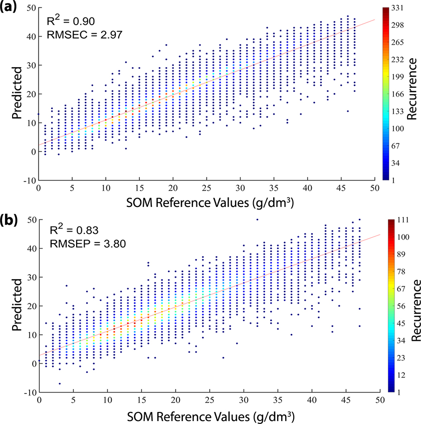
Figure 3. Plot of reference versus predicted values by SVM model in calibration (a) and validation (b) sets.

Analysing the recurrence of the predicted values in Figure 3, it is possible to conclude that most of the samples were predicted with SOM values close to the reference ones. Only a few samples (dark blue) had the predicted values far from the reference values.

This fact can also be observed in Figure 4, which shows the histograms of the prediction errors in calibration and validation sets. The histograms show that most of the samples were predicted with residues of up to 2 × RMSE in both sets, while few samples were predicted with higher residues.

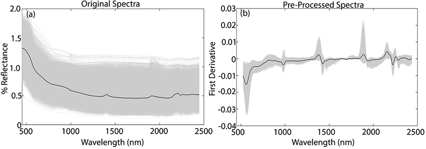
Figure 4. Histograms of the prediction errors in calibration (a) and validation (b) sets.

Conclusions

The support vector machine algorithm was successful in dealing with an extensive and complex soil spectral library to determine SOM content. Brazil’s soils are very diverse and heterogeneous with regards to chemical composition and soil organic matter content. The robustness presented by the proposed methodology involving vis-NIR spectra and machine learning has created high expectations for the possibility of mitigating/eliminating the use of heavy metal reagents in soil fertility analysis. Also, the methodology has potential to be used as a replacement for the traditional method in the future. Knowledge of soil fertility, supported by a green analytical methodology, could pave the way for increasing sustainable agricultural productivity.

Acknowledgements

The authors thank Instituto Nacional de Ciência e Tecnologia de Bioanalítica (INCTBio), Conselho Nacional de Desenvolvimento Científico e Tecnológico (CNPq, Brazil, 465389/2014-7 and 303994/2017-7), Coordenação de Aperfeiçoamento de Pessoal de Nível Superior (CAPES, Brazil, Finance Code 001) and Fundação de Amparo a Pesquisa do Estado de São Paulo (FAPESP, Brazil, 2014/508673) for financial support. We also thank Speclab Holding S.A. for providing the samples and the vis-NIR equipment SpecSoil-Scan^®, and to Embrapa (Project number MP5 14.05.01.001.01.00.00).

References

F.B. de Santana, A.M. de Souza and R.J. Poppi, “Green methodology for soil organic matter analysis using a national near infrared spectral library in tandem with learning machine”, Sci. Total Environ. 658, 895–900 (2019). https://doi.org/10.1016/j.scitotenv.2018.12.263
C. Cortes and V. Vapnik, “Support-vector networks”, Mach. Learn. 20, 273–297 (1995). https://doi.org/10.1023/A:1022627411411
P.R. Filgueiras, J.C.L. Alves, C.M.S. Sad, E.V.R. Castro, J.C.M. Dias and R.J. Poppi, “Evaluation of trends in residuals of multivariate calibration models by permutation test”, Chemometr. Intell. Lab. Syst. 133, 33–41 (2014). https://doi.org/10.1016/j.chemolab.2014.02.002
Mathworks, Statistics and Machine Learning Toolbox ^TM User’s Guide R2017a. MatLab, pp. 1–9214 (2017).
R. Bro and A.K. Smilde, “Principal component analysis”, Anal. Methods. 6, 2812–2831 (2014). https://doi.org/10.1039/c3ay41907j
B. Stenberg, R.A. Viscarra Rossel, A.M. Mouazen, J. Wetterlind, M. Mouazen and J. Wetterlind, “Visible and near infrared spectroscopy in soil science”, Adv. Agron. 107, 163–215 (2010). https://doi.org/10.1016/S0065-2113(10)07005-7
A. Savitzky and M.J.E. Golay, “Smoothing and differentiation of data by simplified least squares procedures”, Anal. Chem. 36, 1627–1639 (1964). https://doi.org/10.1021/ac60214a047